Guerrilla 2018 Classes Now Open

All Guerrilla training classes are now open for registration.

1. GCAP: Guerrilla Capacity and Performance — From Counters to Containers and Clouds
2. GDAT: Guerrilla Data Analytics — Everything from Linear Regression to Machine Learning
3. PDQW: Pretty Damn Quick Workshop — Personal tuition for performance and capacity mgmt

The following highlights indicate the kind of thing you'll learn. Most especially, how to make better use of all that monitoring and load-testing data you keep collecting.

• How to save millions of dollars with a one-line performance model (video)
• How to minimize chargeback after you lift and shift to the cloud (video)
• How to correctly emulate web traffic on a load-testing rig (PDF)

See what Guerrilla grads are saying about these classes. And how many instructors do you know that are available for you from 9am to 9pm (or later) each day of your class?

Who should attend?

• IT architects
• Application developers
• Performance engineers
• Sysadmins (Linux, Unix, Windows)
• System engineers
• Test engineers
• Mainframe sysops (IBM. Hitachi, Fujitsu, Unisys)
• Database admins
• Devops practitioners
• SRE engineers
• Anyone interested in getting beyond performance monitoring

As usual, Sheraton Four Points has bedrooms available at the Performance Dynamics discounted rate. The room-booking link is on the registration page.

Tell a colleague and see you in September!

USL Scalability Modeling with Three Parameters

NOTE: Annoyingly, the remote mathjax server often takes it's sweet time rendering LaTex equations (like, maybe a minute!!!). I don't know if this is deliberate on the part of Google or a bug. It used to be faster. If anyone knows, I'd be interested to hear; especially if there is a way to speed it up. And no, I'm not planning to move to WordPress.

Update of Oct 2018: Wow! MathJax performance is back. Clearly, whinging is the most powerful performance optimizer. :)

The 2-parameter USL model

The original USL model, presented in my GCAP book and updated in the blog post How to Quantify Scalability, is defined in terms of fitting two parameters $\alpha$ (contention) and $\beta$ (coherency). \begin{equation} X(N) = \frac{N \, X(1)}{1 + \alpha \, (N - 1) + \beta \, N (N - 1)} \label{eqn: usl2} \end{equation}

Fitting this nonlinear USL equational model to data requires several steps:

1. normalizing the throughput data, $X$, to determine relative capacity, $C(N)$.
2. equation (\ref{eqn: usl2}) is equivalent to $X(N) = C(N) \, X(1)$.
3. if the $X(1)$ measurement is missing or simply not available—as is often the case with data collected from production systems—the GCAP book describes an elaborate technique for interpolating the value.

The motivation for a 2-parameter model arose out of a desire to meet the twin goals of:

1. providing each term of the USL with a proper physical meaning, i.e., not treat the USL like a conventional multivariate statistical model (statistics is not math)
2. satisfying the von Neumann criterion: minimal number of modeling parameters

Last year, I realized the 2-paramater constraint is actually overly severe. Introducing a third parameter would make the statistical fitting process even more universal, as well as simplify the overall procedure. For the USL particularly, the von Neumann criterion should not be taken too literally. It's really more of a guideline: fewer is generally better.

How to Remember the Poisson Distribution

The Poisson cumulative distribution function (CDF) \begin{equation} F(α,n) = \sum_{k=0}^n \dfrac{α^k}{k!} \; e^{-α} \label{eqn:pcdf} \end{equation} is the probability of at most $n$ events occurring when the average number of events is α, i.e., $\Pr(X \le n)$. Since \eqref{eqn:pcdf} is a probability function, it cannot have a value greater than 1. In R, the CDF is given by the function ppois(). For example, with α = 4 the first 16 values are

> ppois(0:15,4)
 [1] 0.01831564 0.09157819 0.23810331 0.43347012 0.62883694 0.78513039 0.88932602 0.94886638
 [9] 0.97863657 0.99186776 0.99716023 0.99908477 0.99972628 0.99992367 0.99998007 0.99999511

As the number of events increases from 0 to 15 the CDF approaches 1. See Figure.

Importing an Excel Workbook into R

The usual route for importing data from spreadsheet applications like Excel or OpenOffice into R involves first exporting the data in CSV format. A newer and more efficient CRAN package, called XLConnect (c. 2011), facilitates reading an entire Excel workbook and manipulating worksheets and cells programmatically from within R.

XLConnect doesn't require a running installation of Microsoft Excel or any other special drivers to be able to read and write Excel files. The only requirement is a recent version of a Java Runtime Environment (JRE). Moreover, XLConnect can handle older .xls (BIFF) as well as the newer .xlsx (Office XML) file formats. Internally, XLConnect uses Apache POI (Poor Obfuscation Implementation) to manipulate Microsoft Office documents.

As a simple demonstration, the following worksheet, from a Guerrilla Capacity Planning workbook, will be displayed in R.

First, the Excel workbook is loaded as an R object:

Melbourne's Weather and Cross Correlations

During a lunchtime discussion among recent GCaP class attendees, the topic of weather came up and I casually mentioned that the weather in Melbourne, Australia, can be very changeable because the continent is so old that there is very little geographical relief to moderate the prevailing winds coming from the west.

In general, Melbourne is said to have a mediterranean climate, but it can also be subject to cold blasts of air coming up from Antarctic regions at any time, but especially during the winter. Fortunately, the island state of Tasmania acts as something of a geographical barrier against those winds. Understanding possible relationships between these effects presents an interesting exercise in correlation analysis.

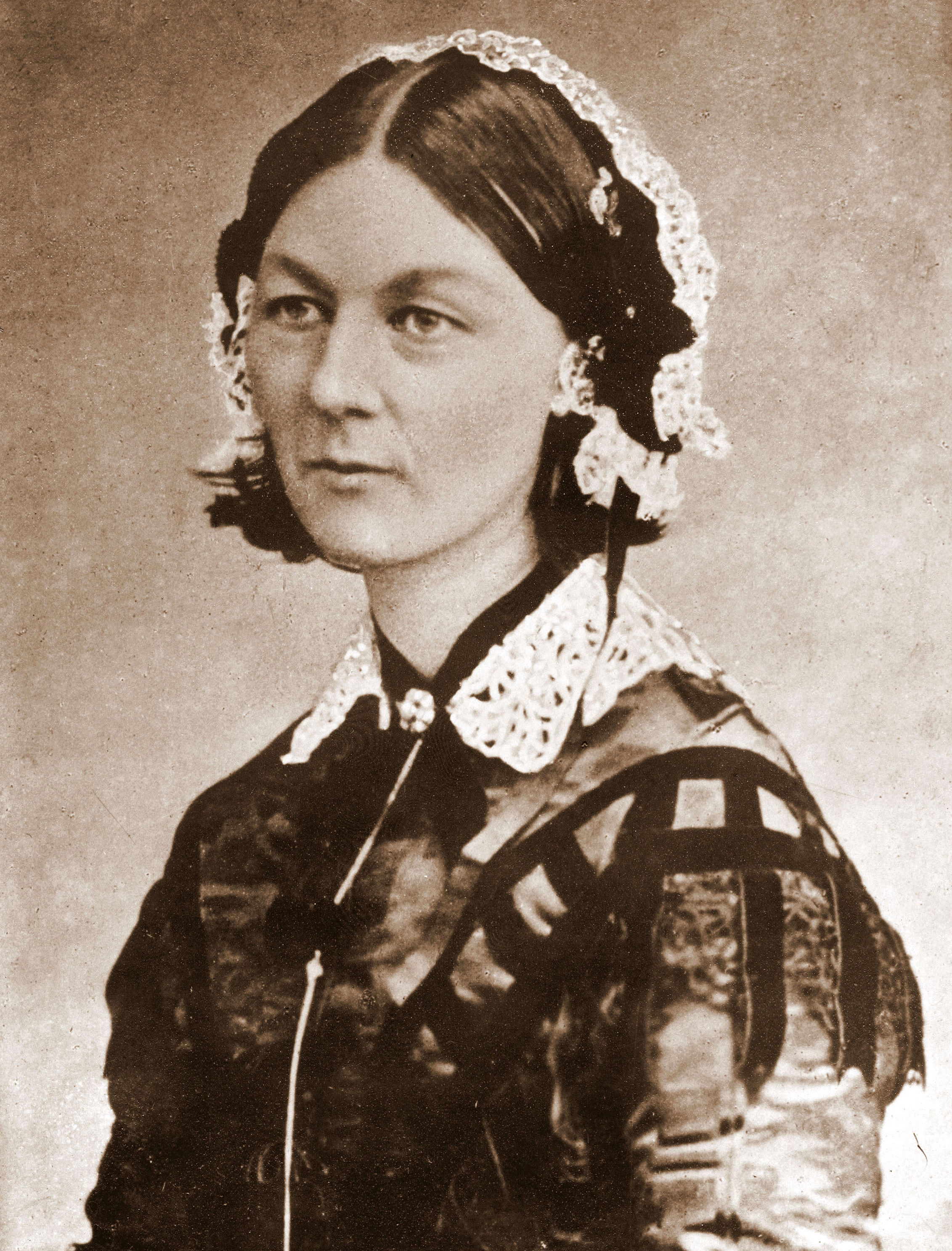
Facebook Meets Florence Nightingale and Enrico Fermi

Highlighting Facebook's mistakes and weaknesses is a popular sport. When you're the 800 lb gorilla of social networking, it's inevitable. The most recent rendition of FB bashing appeared in a serious study entitled, Epidemiological Modeling of Online Social Network Dynamics, authored by a couple of academics in the Department of Mechanical and Aerospace Engineering (???) at Princeton University.

They use epidemiological models to explain adoption and abandonment of social networks, where user adoption is analogous to infection and user abandonment is analogous to recovery from disease, e.g., the precipitous attrition witnessed by MySpace. To this end, they employ variants of an SIR (Susceptible Infected Removed) model to predict a precipitous decline in Facebook activity in the next few years.

Channeling Mark Twain^†, FB engineers lampooned this conclusion by pointing out that Princeton would suffer a similar demise under the same assumptions.

Irrespective of the merits of the Princeton paper, I was impressed that they used an SIR model. It's the same one I used, in R, last year to reinterpret Florence Nightingale's zymotic disease data during the Crimean War as resulting from epidemic spreading.

Another way in which FB was inadvertently dinged by incorrect interpretation of information—this time it was the math—occurred in the 2010 movie, "The Social Network" that tells the story of how FB (then called Facemash) came into being. While watching the movie, I noticed that the ranking metric that gets written on a dorm window (only in Hollywood) is wrong! The correct ranking formula is analogous to the Fermi-Dirac distribution, which is key to understanding how electrons "rank" themselves in atoms and semiconductors.

---

^†"The reports of my death have been greatly exaggerated."

Response Time Percentiles for Multi-server Applications

In a previous post, I applied my rules-of-thumb for response time (RT) percentiles (or more accurately, residence time in queueing theory parlance), viz., 80th percentile: $R_{80}$, 90th percentile: $R_{90}$ and 95th percentile: $R_{95}$ to a cellphone application and found that the performance measurements were not completely consistent. Since the relevant data only appeared in a journal blog, I didn't have enough information to resolve the discrepancy; which is ok. The first job of the performance analyst is to flag performance anomalies but most probably let others resolve them—after all, I didn't build the system or collect the measurements.

More importantly, that analysis was for a single server application (viz., time-to-first-fix latency). At the end of my post, I hinted at adding percentiles to PDQ for multi-server applications. Here, I present the corresponding rules-of-thumb for the more ubiquitous multi-server or multi-core case.

Single-server Percentiles

First, let's summarize the Guerrilla rules-of-thumb for single-server percentiles (M/M/1 in queueing parlance): \begin{align} R_{1,80} &\simeq \dfrac{5}{3} \, R_{1} \label{eqn:mm1r80}\\ R_{1,90} &\simeq \dfrac{7}{3} \, R_{1}\\ R_{1,95} &\simeq \dfrac{9}{3} \, R_{1} \label{eqn:mm1r95} \end{align} where $R_{1}$ is the statistical mean of the measured or calculated RT and $\simeq$ denotes approximately equal. A useful mnemonic device is to notice the numerical pattern for the fractions. All denominators are 3 and the numerators are successive odd numbers starting with 5.

Laplace the Bayesianista and the Mass of Saturn

I'm reviewing Bayes' theorem and related topics for the upcoming GDAT class. In its simplest form, Bayes' theorem is a statement about conditional probabilities. The probability of A, given that B has occurred, is expressed as: \begin{equation} \Pr(A|B) = \dfrac{\Pr(B|A)\times\Pr(A)}{\Pr(B)} \label{eqn:bayes} \end{equation} In Bayesian language, $\Pr(A|B)$ is called the posterior probability, $\Pr(A)$ the prior probability, and $\Pr(B|A)$ the likelihood (essentially a normalization factor).

Source: Wikipedia

Adding Percentiles to PDQ

Pretty Damn Quick (PDQ) performs a mean value analysis of queueing network models: mean values in; mean values out. By mean, I mean statistical mean or average. Mean input values include such queueing metrics as service times and arrival rates. These could be sample means. Mean output values include such queueing metrics as waiting time and queue length. These are computed means based on a known distribution. I'll say more about exactly what distribution, shortly. Sometimes you might also want to report measures of dispersion about those mean values, e.g., the 90th or 95th percentiles.

Percentile Rules of Thumb

In The Practical Performance Analyst (1998, 2000) and Analyzing Computer System Performance with Perl::PDQ (2011), I offer the following Guerrilla rules of thumb for percentiles, based on a mean residence time R:

• 80th percentile: p80 ≃ 5R/3
• 90th percentile: p90 ≃ 7R/3
• 95th percentile: p95 ≃ 9R/3

I could also add the 50th percentile or median: p50 ≃ 2R/3, which I hadn't thought of until I was putting this blog post together.

The Most Important Scatterplot Since Hubble?

In 1929, the astronomer Edwin Hubble published the following scatterplot based on his most recent astronomical measurements.

Figure 1. Edwin Hubble's original scatterplot

It shows the recession velocity of the "stars" (in km/s) on the y-axis and their corresponding distance (in Megaparsecs) on the x-axis. A Megaparsec is about 3.25 million light-years. This scatterplot is important for several reasons:

Harmonic Averaging of Monitored Rate Data

The following slides constitute evolving notes made in response to remarks that arose during the Monitorama Conference in Boston MA, March 28-29, 2013. Since they are evolving, the content will be updated continuously in place. So, get on RSS or Twitter or check back often to read the latest version.

During the Graphite workshop session at Monitorama, the topic of aggregating monitored rate data came up. This caused me to interject the cautionary comment:

Monitorama 2013 Conference

Here is my Keynote presentation that opened the first Monitorama conference and hackathon in Cambridge MA yesterday:

Comments from the #monitorama Twitter stream:

Extracting the Epidemic Model: Going Beyond Florence Nightingale Part II

This is the second of a two part reexamination of Florence Nightingale's data visualization based on her innovative cam diagrams (my term) shown in Figure 1.

Figure 1. Nightingale's original cam diagrams (click to enlarge)

Recap

In Part I, I showed that FN applied sectoral areas, rather than a pie chart or conventional histogram, to reduce the visual impact of highly variable zymotic disease data from the Crimean War. She wanted to demonstrate that diminishing disease was due mostly to her sanitation methodologies. The square-root attenuation of magnitudes, arising from the use of sectoral areas, helped her accomplish that objective. In addition, I showed that a plausibly simpler visualizaiton could have been had with a single 24-month cam diagram. See Fig. 2.

Figure 2. Combined 24-month cam diagram

Going Beyond Florence Nightingale's Data Diagram: Did Flo Blow It with Wedges?

In 2010, I wrote a short blog item about Florence Nightingale the statistician, solely because of its novelty value. I didn't even bother to look closely at the associated graphic she designed, but that's what I intend to do here. In this first installment, I reflect on her famous data visualization by reconstructing it with the modern tools available in R. In part two, I will use the insight gained from that exercise to go beyond data presentation to potentially more revealing data modeling. Interestingly, I suspect that much of what I will present could also have been accomplished in Florence Nightingale's day, more than 150 years ago, albeit not as easily and not by her alone.

Figure 1. Nightingale and her data visualization (click to enlarge)

Although Florence Nightingale was not formally trained as a statistician, she apparently had a natural aptitude for mathematical concepts and evidently put a lot of thought into presenting the import of her medical findings in a visual way. Click on Figure 1 to enlarge it and view the details in her original graphic. As a consequence, she was elected the first female member of the Royal Statistical Society in 1859 and later became an honorary member of the American Statistical Association.

Why Wedges?

Why did FN bother to construct the data visualization in Figure 1? If you read her accompanying text, you see that she refers to the sectors as wedges. In a nutshell, her point in devising Figure 1 was to try and convince a male-dominated, British bureaucracy that better sanitary methods could seriously diminish the adverse impact of preventable disease amongst military troops on the battlefield. The relative size of the wedges is intended to convey that effect. Later on, she promoted the application of the same sanitation methodologies to public hospitals. She was using the established term of the day, zymotic disease, to refer to epidemic, endemic, and contagious diseases.

The Social Network Ranking is Wrong

Call me old-fashioned, but I never saw the 2010 movie The Social Network until last year (at a private screening). In case you also missed it, it's the Hollywood version of how Facebook.com came into being.

Quite apart from any artistic criticisms, I have a genuine psychological problem with movies like TSN. I keep getting caught up in technical inaccuracies and tend to lose the plot. So, it's very hard for me to watch such movies as the director intended. It's the same reason I can't stand SciFi movies or books: I can't get past the impossible and the just plain wrong. It turns out that TSN is generally fairly accurate regarding things like Linux, MySQL, PHP, and so forth, but there is a real clanger: the ranking algorithm used by Facemash—the Facebook precursor.

There's a scene where the Mark Zuckerberg character wants to rank Harvard women based on crowd-sourced scores. He recalls that his best friend (at the time), Eduardo Saverin, had previously mentioned a ranking formula, but Zuck can't remember how it goes, so he can't code it. When Saverin shows up again, Zuck urgently asks him to reveal it. In typical Hollywood style—possibly to keep a generally math-phobic audience visually engaged—Saverin writes the ranking equations on the dorm window (see above image) for the desperate Zuckerberg. Where else would you write equations?

Here they are, reproduced with a little better formatted: \begin{align} Ea &= \dfrac{1}{1 + 10 (Rb-Ra)/400}, & Eb &= \dfrac{1}{1 + 10 (Ra-Rb)/400} \label{eqn:movie} \end{align} There's just one slight problem: they're wrong!

Visualizing Variance

The typical presentation of variance in textbooks often looks like this Wikipedia definition. Quite daunting for the non-expert. So, how would you explain the notion of variance to someone who has little or no background in statistics and couldn't easily digest all that gobbledygook?

The Mean

Let's drop back a notch. How would you explain the statistical mean? A common way to do that is to utilize the simple visual device of the "bell curve" belonging to the normal distribution (Fig. 1).

Figure 1. A normal distribution

The normal distribution, $N(x,\mu,\sigma^2)$, is specified by two parameters:

1. Mean, usually denoted by $\mu$
2. Variance, usually denoted by $\sigma^2$

that determine (1) the location and (2) the shape of the curve. In Fig. 1, $\mu = 4$. Being a probability, the curve must be normalized to enclose unit area. Also, since $N(x)$ is unimodal and symmetric about $\mu$, the mean, median and mode are all located at the same position on the $x$-axis. Therefore, it's easy to point to the mean as being the $x$-position of the peak. Anybody can see that immediately. Mission accomplished.

But what about the variance? Where is that in Figure 1?

PDQ 6.0 is On Its Way

PDQ (Pretty Damn Quick) version 6.0.β is in the QA pipeline. Although this is a major release, cosmetically, things won't look any different when it comes to writing PDQ models. All the big changes have taken place under the hood in order to make PDQ more consistent with the R statistical environment.

R version 2.15.2 (2012-10-26) -- "Trick or Treat"
Copyright (C) 2012 The R Foundation for Statistical Computing
ISBN 3-900051-07-0
Platform: i386-apple-darwin9.8.0/i386 (32-bit)

> library(pdq)
> source("/Users/njg/PDQ/Test Suites/R-Test/mm1.r")
                ***************************************
                ****** Pretty Damn Quick REPORT *******
                ***************************************
                ***  of : Thu Nov  8 17:42:48 2012  ***
                ***  for: M/M/1 Test                ***
                ***  Ver: PDQ Analyzer 6.0b 041112  ***
                ***************************************
                ***************************************
...

The main trick is that the Perl and Python versions of PDQ will remain entirely unchanged while at the same time invisibly incorporating significant changes to accommodate R.

Load Testing with Uniform vs. Exponential Arrivals

In a couple of recent blog posts about generating exponential loads and why that is important for load testing and performance testing, it was not completely clear to some readers what was motivating my remarks. In this post, I will try to provide a more visual elaboration of that aspect.

My fundamental point is this. When it comes to load testing^*, presumably the idea is to exercise the system under test (SUT). Otherwise, why are you doing it? Part of exercising the SUT is to produce significant fluctuations in the number of requests residing in application buffers. Those fluctuations can be induced by the pattern of arriving requests issued by the client-side driver (DVR): usually implemented as a pile of PCs or blades.

On the Accuracy of Exponentials and Expositions

The following is a slightly edited version of my response to a Discussion on the Linkedin CPPE group, which is accessible to Members Only. It's written in the style of a journal reviewer. The original Discussion topic was based on a link to a blog-post. I've been asked to make my Linkedin review more widely available so, here tiz...

The blog-post Capacity Planning on a Cocktail Napkin is a really good example of a really bad explanation. There are so many things that are misleading, at best, and flat-out wrong, at worst, it's hard to know where to begin (or where to stop). Nevertheless, I'll try to keep it brief [I failed in that endeavor. — njg].

The author applies the equation:

\begin{equation} E = λ \end{equation}

Why? What is that equation? We don't know because the author does not say yet what all the symbols mean. It's all very well to impress people by slinging equations around, but it's more important to say what the equations actually mean. After all, the author might have chosen the wrong one.

Visual Illusions: Google vs Facebook vs Yahoo

The ability to visualize data, enabled by the advent of graphical computer tools, has been a great boon to Cap and Perf. The power derives from the way graphical displays provide an efficient impedance match to the visual system in our brain. The weakness derives from the way graphical displays provide an efficient impedance match to the visual system in our brain. We can get carried away by visual representations alone. Every marketing organization exploits that weakness. Numbers do have poor cognitive impedance, but that doesn't mean numbers should ignored altogether. In fact, we often need a combination of both numerical and visual data representations so that we don't suffer visual miscues and thus jump to the wrong conclusion. The following presents an example of how easily this can happen.

Recently, Guerrilla alumnus, Scott J. pointed me at this Chart of the Day showing how Google revenue growth was outpacing both Facebook and Yahoo, when compared 7 years after launching the respective companies.

Clearly, this chart is intended to be an attention getter for the Silicon Alley Insider website but, it looks about right and normally I might have just accepted the claim without giving it anymore thought. The notion that Google growth is dominating, is also consistent with a lot of other things one sees. No surprises there.