Sex, Lies and Log Plots

From time to time, at the Hotsos conferences on Oracle performance, I've heard the phrase, "battle against any guess" (BAAG) used in presentations. It captures a good idea: eliminate guesswork from your decision making process. Although that's certainly a laudable goal, life is sometimes not so simple; particularly when it comes to performance analysis. Sometimes, you really can't seem to determine unequivocally what is going on. Inevitably, you are left with nothing but making a guess—preferably an educated guess, not a random guess (the type BAAG wants to eliminate). As I say in one of my Guerrilla mantras: even wrong expectations (or a guess) are better than no expectations. In more scientific terms, such an educated guess is called a hypothesis and it's a major way of making scientific progress.

Of course, it doesn't stop there. The most important part of making an educated guess is testing its validity. That's called hypothesis testing, in scientific circles. To paraphrase the well-known Russian proverb, in contradistinction to BAAG: Guess, but justify^*. Because all hypothesis testing is a difficult process, it can easily get subverted into reaching the wrong conclusion. Therefore, it is extremely important not to set booby traps inadvertently along the way. One of the most common visual booby trap arises from the inappropriate use of logarithmically-scaled axes (hereafter, log axes) when plotting data.

Linear scale:

Each major interval has a common difference $(d)$, e.g., $200, 400, 600, 800, 1000$ if $d=200$:

Log scale:

Each major interval has a common multiple or base $(b)$, e.g., $0.1, 1, 10, 100, 1000$ if $b=10$:

The general property of a log axis is to stretch out the low end of the axis and compress the high end. Notice the unequal minor interval spacings. Hence, using a log scaled axis (either $x$ or $y$) is equivalent to applying a nonlinear transformation to the data. In other words, you should be aware that introducing a log axis will distort the visual representation of the data^†, which can lead to entirely wrong conclusions.

GCaP Class: Sawzall Optimum

In a side discussion during last week's class, now Guerrilla alumnus, Greg S. (who used to work at Google a few years ago) informed me that typical Sawszall preprocessing-setup times typically lie in the range from around 500 ms to about 10 seconds, depending on such factors as: cluster location, GFS chunkserver hit rate, borglet affinity hits, etc. This is the information that was missing in the original Google paper and prevented me from finding the optimal machine configuration in my previous post.

To see how these new numbers can be applied to estimating the corresponding optimal configuration of Sawzall machines, let's take the worst case estimate of 10 seconds for the preprocessing time. First, we convert 10 s to 10/60 = 0.1666667 min (original units) and plot that constant as the horizontal line (gray) in the lower part to the figure at left (click to enlarge). Next, we extend the PDQ elapsed-time model (blue curve) until it intersects the horizontal line. That point is the optimum, as I explained in class, and it occurs at p = 18,600 machines (vertical line).

That's more than thirty times the number of machines reported in the original Google paper—those data points appear on the left side of the plot. Because of the huge scale involved, it is difficult to see the actual intersection, so the figure on the right shows a zoomed-in view of the encircled area. Increasing the number of parallel machines beyond the vertical line means that the elapsed time curve (blue) goes into the region below the horizontal line. The horizontal line represents the fixed preprocessing time, so it becomes the system bottleneck as the degree of parallelism is increased. Since the elapsed times in that region would always be less than the bottleneck service time, they can never be realized. Therefore, adding more parallel machines will not improve response time performance.

Conversely, a shorter preprocessing time of 500 ms (i.e., a shorter bottleneck service time) should permit a higher degree of parallelism.

Scalability of Sawzall, MapReduce and Hadoop

This is a follow-up to a reader comment by Paul P. on my previous post about MapReduce and Hadoop. Specifically, Paul pointed me at the 2005 Google paper entitled "Parallel Analysis with Sawzall," which states:

"The set of aggregations is limited but the query phase can involve more general computations, which we express in a new interpreted, procedural programming language called Sawzall^†"

† Not related to the portable reciprocating power saw manufactured by the Milwaukee Electric Tool Corporation.

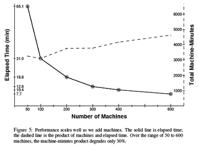
More important, for our purposes, is Section 12 Performance. It includes the following plot, which tells us something about Sawzall scalability; but not everything.

Figure 1.