
Waiting costs money
As is often the case, this is yet another example of business management types applying queueing theory to solve problems which, when looked at askew, have fairly obvious applications to computer performance analysis. In this case, Liao considers the financial impact on retailers of queueing at places like fast food restaurants, banks, postal services, toll plazas and even buying tickets for a theme park ride. More particularly, he examines the losses in revenue due to customers who either balk or reneg from a queue.
The author notes that just a 1% balking rate at drive-thru restaurants can reduce revenue by more than $100 million per annum for each $10 billion in sales. The similarities with lost revenue due to frustrated web users and the cost of dynamic resource allocation in cloud computing should be apparent.
The revenue impact of slow web services was a hot topic at Velocity 2009. For example, if Amazon.com adds a feature to their website and it ends up causing an increase of just 100 milliseconds in end-user latency, they sell 1% fewer books. That equates to something like $200 million in lost revenue. An attempt to combine dollar-costs with performance metrics for cloud computing arose out of attending another Velocity 2009 presentation so, I'm looking forward to a continuation of this topic at Velocity 2010.
Balking and reneging losses
In queue-theoretic parlance, balking means that an arriving customer already considers the waiting line to be too long and aborts the mission before joining the queue. In terms of a queueing diagram, balking can be represented as shown in figure (a). Reneging means that the customer decides to abort the mission after having already joined the queue. Diagrammatically, this is shown in figure (b).
 |
|
| (a) Balking | (b) Reneging |
The way this is handled in queueing theory is to assign a probability for either balking or reneging, which the author denotes θ1 and θ2, respectively and these probabilities are the ones referred to in the PhysOrg article. They both need to be determined empirically and Liao describes an example showing how this can be achieved using data collected at 15 minute intervals—just like we do for computer systems. Without going into the details, I'm just going to construct a PDQ-R model to reproduce the author's main result, which can be described as follows.
We anticipate that a higher balking probability is associated with a mean queue length that is shorter than it would be otherwise, and a higher reneging probability is associated with a shorter mean waiting time. However, that also means a corresponding loss of revenue—as in, no sale! To reduce the likelihood of balking and reneging, the retail manager could add more service resources, i.e., cashiers, to ensure a shorter waiting line, but cashiers cost money in terms of wages. So, too few service resources (servers) and you lose revenue due to balking and reneging; too many servers and your operational costs increase. It's a tradeoff and the capacity planning question becomes: What is the optimal service configuration?
PDQ model in R
To find the optimal server configuration, I've set up a PDQ model in R using the same modeling assumptions as the author. Based on the existing literature, Liao tells us that many retail facilities are commonly represented as M/M/m queues. I'll call the balking probability pB and the reneging probability pR in this PDQ model. Here is a list of the parameters taken straight out of Liao's 2007 paper.
library(pdq)

pB <- 0.0081    # prob of balking
pR <- 0.0220    # prob of reneging
A  <- 100       # mean spend/cust in dollars
R  <- 0.5       # net profit/cust in dollars
K  <- 90        # cost of server/hr in dollars
aRate <- 147    # cust/hour
sRate <- 40     # cust/hour
minServers <- 4
maxServers <- 10
costServ   <- 0
costBLoss  <- 0
costRLoss  <- 0
costTotal  <- 0
Next, I construct the PDQ queueing model and solve it for the performance metrics of interest, viz., the waiting-line length (Lq) and the waiting time (Wq). Since we want the cost as a function of the number of cashiers (m) in the retail facility, I set up a loop over the number of servers (m) using the CreateMultiNode() function to represent each M/M/m queue configuration.
for(m in minServers:maxServers) {
Init("")
CreateOpen("customers",aRate)
CreateMultiNode(m,"cashier",CEN,FCFS)
SetDemand("cashier","customers",1/sRate)
Solve(CANON)

Lq <- GetQueueLength("cashier","customers",TRANS) - aRate/sRate

Wq <- 60 * Lq/aRate
numBalk  <- Lq * pB * aRate
numReneg <- Wq * pR * aRate
costServ[m]  <- m * K
costBLoss[m] <- numBalk  * A * R
costRLoss[m] <- numReneg * A * R
costTotal[m] <- costServ[m] + costBLoss[m] + costRLoss[m]
}
Finally, I plot the collected performance metrics computed by the PDQ model.
plot(costTotal,xlim=c(minServers,maxServers),type="b",col="red",lwd=2,
main="Cost of Elastic Capacity Demand",xlab="Servers (m)",ylab="Cost ($)")
lines(costServ,xlim=c(minServers,maxServers),type="b",col="blue",lty="dashed")
lines(costBLoss,xlim=c(minServers,maxServers),type="b",lty="dashed")
lines(costRLoss,xlim=c(minServers,maxServers),type="b",lty="dashed")
arrows(x0=6,y0=800,x1=6,y1=600)
text(6,850,"minimum cost")
text(4.5,1200,"operational cost",adj=c(0,0))
text(7,550,"service cost",adj=c(0,0))
text(7,90,"balking and reneging losses",adj=c(0,0))
Now, we're in a position to assess the financial impact of adding capacity on-demand.
Capacity-cost analysis
The following plot generated by the above PDQ-R model displays the dollar cost on the y-axis as a function of the elastically assigned server capacity on the x-axis. Immediately, we see that the lowest total cost occurs at m = 6 cashiers with the above set of retail-facility parameters.

This makes sense because the increased parallelism due to more servers has the effect of reducing the queue length, and therefore the losses due to balking and reneging (black dashed curves). In fact, for this set of parameter values, there's not much distinction between balking and reneging losses. Since these curves fall as 1/m, they are hyperbolic in form. We've seen similar hyperbolic curves before in my analysis of Google's Sawzall scalability, except the number of servers in that case was astronomical.
On the other hand, the cost of adding servers (something the Google paper didn't discuss) increases linearly with m (blue dashed line in the above plot). The total cost (red curve) is the sum of all these contributions. Although the reduction in balking and reneging losses wins when a small number of servers are added, the total cost becomes dominated by server cost for larger configurations.
Too many cooks cost
Finally, it's worth noting the similarity between the red cost curve and the latency curve associated with Brooks' law: Adding more manpower to an already late software project just makes it later; which I discussed previously from the standpoint of its relationship to my universal scalability law (USL) . There I showed that the principle of Brooks' law is contained in the following USL latency diagram.
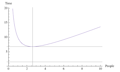
Of course, Brooks didn't present any mathematical analysis, but it's clear that the associated latency function also has a minimum. In that blog post, I showed that this latency or schedule delay (as Brooks would think of it) is specifically due to one-on-one conversations, or pairwise exchange of information, between the existing programmers and the new programmers added to the project. With a small number of added programmers, there's a benefit but, add too many and the conversational overhead kills the delivery schedule. In the context of the USL, the same effect causes poor multicore scalability. In business management lingo, we would say that productivity falls with the increasing number resources, i.e., a negative return on investment!
What Liao has done is show how revenue losses can be formally associated with conventional performance metrics, like queue length or user waiting-time, and this connection becomes very important when service resources are incrementally reallocated according to demand. Without proper provisioning and accounting both providers and users can be nickel and dimed to death.
6 comments:
The dimension of the numBalk parameter does not look to be correct unlike the numReneg parameter (I expected both to be dimensionless). Has numBalk (numBalk <- Lq * pB * aRate) been correctly defined ?
Excellent question and well spotted!
Since this isn't my work, I have a few questions of my own but missed that one. I'll take another look at it but if I can't resolve it, I'll try contacting the author. Stay tuned.
Well, it turns out that I did spot it, but numerically rather than dimensionally (as Raja did).
If you look in the second box of my R code, midway I have written Little's law as Wq <- 60 * Lq/aRate. That 60 is the measurement period T = 60 minutes. So, the quantity that goes into numReneg is actually Wq/T, rather than just Wq, and that makes it dimensionless, just as Raja noticed it should be.
Originally, I ran into problems because I didn't get the same Wq numbers that the author tabulated. I noticed that I could correct them with a factor of 60 and recognized that stood for the T period.
Liao's discussion of numReneg is incorrect for this same reason, but I really hadn't completely corrected all this in my mind until now.
Once again, excellent observation, Raja. Thanks.
Neil, thanks for your time to answer my question. So, it looks like Liao's definition of the numBalk parameter is then incorrect.
I would put it this way. I haven't seen the latest paper because it wasn't accessible on the web, but the 2007 discussion is sloppy. However, because all the calculations are done wrt T = 60 min intervals, it all comes out in the wash. I see no reason to suspect that his main conclusions are wrong.
Post a Comment