
My fundamental point is this. When it comes to load testing*, presumably the idea is to exercise the system under test (SUT). Otherwise, why are you doing it? Part of exercising the SUT is to produce significant fluctuations in the number of requests residing in application buffers. Those fluctuations can be induced by the pattern of arriving requests issued by the client-side driver (DVR): usually implemented as a pile of PCs or blades.
All of the most commonly employed load-test harnesses (e.g., LoadRunner, JMeter) do not facilitate the production of significant variation in the arrival pattern. By default, they only offer a uniform distribution of delays† between the completion of one request and the commencement of the next. This delay is typically set as the think-time value in the client-side script. Consequently, the times between requests arriving at the SUT follows a uniform pattern or uniform distribution. By way of comparison, Figure 1 shows that a better choice for creating greater variation in the interarrival periods is associated with an exponential distribution‡. But Figure 1 only offers a visual clue. We need to quantify the performance insights gained from this exponential burstiness.

Figure 1. Patterns produced by uniform (blue) and exponential (red) arrival instants (vertical notches) in continuous time (horizontal lines). Uniform arrivals resemble regularly spaced plot-axis graduations, whereas exponential arrivals exhibit clumping or bursts in time.
There are many reasons why an exponential arrival pattern is desirable:
- Unlike the uniform distribution, the exponential distribution is asymmetric about its mean.
- It exhibits more burstiness, even though it is random. (cf. Fig. 1)
- By comparison, buffer occupancy in the SUT will reach a higher level.
- Higher occupancy will be observed as longer response times.
- Load tests and stress tests can better detect buffer overflow conditions.
- Performance measurements can be more conveniently validated with other performance analysis tools, e.g., PDQ.
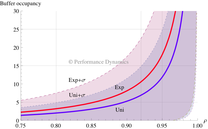
Figure 2. Calculated buffer occupancy as a function of SUT load for uniform and exponential arrivals. The solid curves represent the average occupancy and the shaded regions correspond to the standard deviation intervals about the respective means.
For our purposes, we'll assume the buffer in Figure 2 is the one that receives incoming requests from the load-test driver. The x-axis represents the SUT load $\rho$ ranging between 75% and 100% busy, i.e., high-load conditions and the y-axis is the corresponding number of requests in the buffer.
First, note the location of the solid blue and red curves on the plot. The red curve, which belongs to exponential (Exp) arrivals at the SUT, is sitting above the blue curve, which belongs to uniform (Uni) arrivals. These curves represent the average occupancy of the buffer due to the corresponding arrival pattern. Suppose a buffer occupancy of 5 requests (horizontal line in Fig. 2) in the SUT corresponds to an acceptable average response time. That service level would be reached at 85% busy with Exp arrivals but would not be reached until almost 90% load with Uni arrivals. For heavy loads, even a 5% increase in SUT utilization could necessitate running many more client scripts with a Uni arrivals pattern.
Of course, the solid curves only represent the average buffer occupancy and the difference between Uni and Exp arrivals would most likely show up in the respective measured response times. More importantly, however, if the buffer was designed for a maximum occupancy of 5 requests, that overflow condition would be reached even earlier due to fluctuations in the arrival pattern.
Specifically, the dotted line (above the red curve) reaches that buffer limit at 80% busy, whereas the dashed line (above the dotted line) reaches that limit before 75% busy. The dotted line corresponds to one standard deviation above the Uni mean (denoted $\text{Uni}+\sigma$ in the plot) while the dashed line (i.e., $\text{Exp}+\sigma$) corresponds to one standard deviation above the Exp mean. The standard deviation being the square root of the variance is the classic measure of fluctuations in statistics.
One standard deviation below each of the Uni and Exp solid curves is represented by the regions extending toward the lower right of Figure 2.§ The two regions (corresponding to $\text{Uni}-\sigma$ and $\text{Exp}-\sigma$) overlap so much that the dotted boundary (innermost) and the dashed boundary (outermost) are almost indistinguishable. Although this region might be of less interest generally, it is still part of the information about arrival fluctuations. Keep in mind that the deviations from the respective mean occupancy values must be read vertically.
Finally, it should be quite apparent from Figure 2 that the mean of the Exp distribution taken together with its corresponding fluctuations completely subsumes the mean and the standard deviations of the Uni distribution for all possible SUT loads. Indeed, one could generalize this discussion to consider distributions that offer even more variation in arrival patterns than does the Exp distribution. That's why it would be nice to have a comprehensive library of variate generators included with the load testing harness‡.
Postscript
Being able to select different think time distributions is an important control parameter for specifying a load test. In the past week, I managed to establish a new result that presents yet another subtle twist on the above discussion.The choice of think-time distribution has no effect on mean queue lengths or the mean response time of the SUT, if the load test is emulating a fixed number of users. By default, this is probably the most common type of load test setting where each user (i.e., LR vuser or load generator) cannot issue more than one outstanding request at a time. That also means there is one less performance control parameter available for specification in the requirements for this type of test.
Conversely, the choice of think-time distribution does have a very significant effect on queue lengths and response times in a load-test simulation of internet or web applications. That's the kind of workload assumed in the above post. I'll say more about this new insight in my Guerrilla classes.
* Here, I'm using the term "load test" rather generically. I realize there is a distinction between stress testing, load testing, and performance testing. In general, the latter involves many more measurements at a variety of load levels. In lieu of that, performance analysts may be able to steal load test data and make something out of it.
† There is a very simple explanation for the default delay being a uniform distribution. It's the distribution produced by any native (pseudo) random number generator.
‡ I've shown elsewhere (See eqn. (6) there) that it's essentially a 1-liner to convert a uniform distribution to an exponential distribution but the point is, why should you have to? A load-test harness is nothing more than a very complex simulation platform. No self-respecting simulationist would accept an event-based simulator that did not include a library of selectable distributions in the $10K price tag, let alone paying hundreds of thousands of dollars for a load-test harness that has none.
§ Strictly speaking, the extreme lower boundaries in Fig. 2 extend completely into the lower-right corner of the plot, but I've artificially truncated them at 95% of the negative $\sigma$ value in the interest of maintaining visual clarity.
13 comments:
We may not code the exponential delay logic if we use http://binfalse.de/2011/02/talking-r-through-java/
Thanks for the explanation.
Hi Dr. Gunther,
I have 2 questions:
. is it possible to see somewhere also the comparison graph with a deterministic arrival, i.e. exactly 1 request every 1/Lambda seconds? sttdev will be zero.
. Sometimes I have logs that report service times that look exponential distributed, but the curve is translated to the right (most frequent time is greater than 0). Can they still be considered exponential? If I adjust the bin width I can make the most frequent duration fall into the first bucket, making it perfectly exponential, but I don't know if this can be considered illegal cheating.
Thanks
MatteoP
MatteoP, It's not so easy to find comparative curves because they must be calculated numerically. To that end, I've computed the mean buffer sizes including the deterministic arrivals case.
As you might guess, since there are no fluctuations in the arrivals, the mean queue size (green) is lower than for the other distributions. If there were no fluctuations in the SUT service periods either, there would be no queue at all.
MatteoP, Without seeing your data it's hard for me to give a definitive answer. However, from your description, it sounds like direct evidence for the so-called "memoryless" property that also uniquely characterizes the Exp dsn.
See Figure A.1 in my Perl::PDQ book on p.428 of the new edition. There, the original Exp curve with value 1/2 at the origin (x=0) is shifted right such that the value of 1/2 now occurs at x=2. From that it should be clear that the Exp function preserves its shape under time translations. Physically, that means it doesn't matter when we start the measurement process. We still end up with an Exp dsn.
We can prove that it's still an Exp function by projecting the top part of the shifted curve back to the origin (x=0). What we get is just another Exp function with a different (bigger) starting value at the origin.
Wow, it seems that exponential distribution provoke a queue length at least doubled (and so wait time)compared with deterministic one. Very interesting, it is what I was looking to have an idea of how unrealistic would be a test with a deterministic arrival rate.
Thanks.
MatteoP
That's right and that's why I didn't bother with the deterministic case. Moreover, the default for test harnesses is to issue uniform distd arrivals. Why? Because they simply make a call to a pseudo-RNG and the dsn of an RNG is uniform (e.g., return a double b/w 0 and 1).
If you have deterministic service periods as well, then you get a conveyor belt (D/D/1 queue) where all the requests simply clock through the SUT with no waiting time involved.
Only if you overdrive it at 100% busy (on average) do requests pile up. But by then, the queue size becomes instantly unbounded, leading to a permanent buffer overflow condition.
I have a question about the number of runs and confidence intervals. How do we get the number of runs of measurements required generally ? There is a recommended procedure in http://www.cse.iitb.ac.in/~puru/courses/spring12/cs695/downloads/cuttingcorners.pdf
Thanks.
Good question and one that I'll be addressing next week in the GDAT class. For some inexplicable reason, I don't see your name on the list. ???
Here is an example in R that calculates the number of measurements needed for wait-times (e.g., as reported in DBMS stats) at the 90% CI:
wtimes <- c(8.0,7.0,5.0,9.0,9.5,11.3,5.2,8.5)
wtmean <- mean(wtimes)
wtsd <- sd(wtimes)
cipc <- 0.90
alpha <- 1-cipc
tval <- qt(1-alpha/2,df=length(wtimes)-1)
r <- 3.5
n <- (100*tval*wtsd/(r*wtmean))^2
n <- ceiling(n)
Thanks for providing valuable information.
Here i am providing a dofollow forum which discusses on Software Testing topics. Register and start discussions.Also you can get a backlink from this website.
Software Testing Discussion Forum
Postscript added.
Hi Neil
An interesting read and I agree with the theory. I agree that uniform load tests do not mimic reality. On the other hand I wonder if having exponential distribution wouldn't overcomplicate the scenario, specifically when it comes to the consistency of the test results. If each test won't behave close enough to the previous tests results might differ in a way which may prevent you from being able to compare tests. One of the very basics in performance testing is the ability to reproduce and I wonder if your idea doesn't conflict with that ability?
Hi Shmuel. I think we're missing each other.
Uniform does not mean "identical," but uniformly distributed with a mean and variance: usually selected by asserting a think time with some range, in the test script(s). Although you may not be aware of it, the uniform distribution is hidden in the random number generator of the load-test harness. In that sense, none of your current tests are identically repeatable.
Similarly, the Exp distribution has a defined mean and variance, but the variation is larger than the uniform case, which is what would allow you to test the "edges" of the queueing envelope.
On top of all that, the SUT is not a deterministic system anyway, so ALL your measured throughputs and response times have errors in them. They're not reported in any load-test tools that I've seen. In other words, the reported throughput should always be the mean throughput +/- error representation.
Do you know what the size of your measurement errors are? That's one of the things I teach in my GDAT class.
Hi Neil,
You are right with your previous comment.
My point was that with the diff between tests results might get spiky when taking the exponential approach in compare to uniform.
I guess that at the end it comes to the ability to ignore outliers and to have tools to normalize tests results so comparison is made easier.
Post a Comment